Alignment of Microbial Consortia • ramen

Introduction

The alignment system in ramen quantifies how similar two or more microbial communities are from a functional perspective – not by which species are present, but by which metabolite-to-metabolite pathways they catalyse. align() supports three modes: pairwise (two consortia), multiple (all consortia in a set), and search (one query consortium against every member of a set). All three return a ConsortiumMetabolismAlignment (CMA) object containing similarity scores and (depending on the mode) pathway correspondences, a consensus network, or a ranked hit table.

This vignette covers the alignment system in depth. For a general introduction to the package, see vignette("ramen", package = "ramen").

Note on help lookup. If tibble or pillar is loaded in your session, ?align may resolve to pillar::align() first. To view the documentation for this package’s generic, use ?ramen::align.

library(ramen)

Mathematical formulation

This section gives the formal definitions of every quantity computed by align(). Notation follows Hirt (2025), the master’s thesis from which the package originated; equation numbers prefixed (thesis eq. ...) refer to that document.

Notation

Let $\Omega = \{\omega^{(1)}, \dots, \omega^{(n)}\}$ denote a collection of consortia (thesis eq. 1). For one consortium $\omega^{(\alpha)}$ , write $\mathcal{M}^{(\alpha)}$ for its set of metabolites; for two consortia under comparison let $\mathcal{M} = \mathcal{M}^{(\alpha)} \cup \mathcal{M}^{(\beta)}$ with $|\mathcal{M}| = m$ (thesis eq. 3). All assays are square $m \times m$ matrices on this union metabolite space. We write $X = \mathbf{X}^{\mathrm{bin},(\alpha)}$ and $Y = \mathbf{X}^{\mathrm{bin},(\beta)}$ for the two binary assays under comparison; analogous symbols $C_X, P_X, N_X$ denote the Consumption, Production, and nSpecies assays. The $L_1$ norm $\lVert A \rVert_1 = \sum_{i,j} |A_{ij}|$ is the sum of all entries; $A \odot B$ is the elementwise (Hadamard) product.

A pathway in ramen is a directed metabolite-to-metabolite pair $(i, j)$ such that some species in the consortium can consume $i$ and some species (possibly the same one) can produce $j$ . Pathways are not biochemical reactions: they are capabilities inferred from the Cartesian product of each species’ uptake set and secretion set. A consortium of two species, one consuming $\{a, b\}$ and producing $\{c, d\}$ , contributes the four pathways $\{a \to c, a \to d, b \to c, b \to d\}$ from only four distinct exchange events (two uptakes, two secretions). See the Cross-product inflation caveat below.

Assay matrices

Each ConsortiumMetabolism stores eight assays (thesis eq. 1, 2):

Binary $\mathbf{X}^{(\alpha,1)}$ : $X^{(\alpha,1)}_{ij} = 1$ if any species in $\omega^{(\alpha)}$ realises pathway $i \to j$ , else $0$ .
nSpecies $\mathbf{X}^{(\alpha,2)}$ : number of distinct species supporting $i \to j$ .
Consumption $\mathbf{X}^{(\alpha,3)}$ : $F^{(c)}_{ij} = \sum_s f^{(c,s)}_{ij}$ , the summed uptake flux of metabolite $i$ across all species participating in $i \to j$ .
Production $\mathbf{X}^{(\alpha,4)}$ : $F^{(p)}_{ij} = \sum_s f^{(p,s)}_{ij}$ , analogously for secretion.
EffectiveConsumption $\mathbf{X}^{(\alpha,5)}$ and EffectiveProduction $\mathbf{X}^{(\alpha,6)}$ : flux-corrected effective fluxes (see below).
nEffectiveSpeciesConsumption $\mathbf{X}^{(\alpha,7)}$ and nEffectiveSpeciesProduction $\mathbf{X}^{(\alpha,8)}$ : Hill-1 effective number of contributing species (see below).

All eight are constructed as the Cartesian product $\mathrm{consumed}(s) \times \mathrm{produced}(s)$ for each species $s$ , then aggregated across species. This cross-product is the source of the density inflation discussed under Limitations and caveats.

Effective flux and effective species count

For a pathway $(i, j)$ with participating species $s_1, \dots, s_n$ , let $p^{(\phi,s)}_{ij} = f^{(\phi,s)}_{ij} / F^{(\phi)}_{ij}$ be the fraction of total flux of type $\phi \in \{c, p\}$ contributed by species $s$ . The Shannon entropy of this distribution is $H_{ij}^{(\phi)} = -\sum_s p^{(\phi,s)}_{ij} \log_2 p^{(\phi,s)}_{ij}$ , and the Hill-1 perplexity $D_{1,ij}^{(\phi)} = 2^{H_{ij}^{(\phi)}}$ is the effective number of species contributing to the pathway: unitless, $\in [1, n]$ , maximised when all species contribute equally.

ramen exposes both the perplexity itself and the flux-corrected flux $F \cdot D_1$ (thesis eq. 2) as separate assays. They are two views of the same network: $\mathbf{X}^{(\alpha,5)}_{ij} = \mathrm{round}\bigl( F^{(c)}_{ij} \cdot 2^{H^{(c)}_{ij}}, 2 \bigr), \qquad \mathbf{X}^{(\alpha,7)}_{ij} = \mathrm{round}\bigl( 2^{H^{(c)}_{ij}}, 2 \bigr),$ and analogously $\mathbf{X}^{(\alpha,6)}, \mathbf{X}^{(\alpha,8)}$ for production. EffectiveConsumption and EffectiveProduction carry the same units as Consumption / Production (a flux, larger when total flux is large and species contribute evenly); nEffectiveSpeciesConsumption and nEffectiveSpeciesProduction are unitless counts mirroring nSpecies. The algebraic identity $\mathbf{X}^{(\alpha,5)} = \mathbf{X}^{(\alpha,3)} \odot \mathbf{X}^{(\alpha,7)}$ holds cell-wise (modulo two-decimal rounding); same for production. See the Hill-1 saturation caveat for behaviour on small consortia.

Pairwise alignment metrics

Throughout, $X$ and $Y$ are binary assays expanded to the union metabolite space, and $C_X, P_X, N_X$ are the Consumption, Production, and nSpecies assays for consortium $X$ .

FOS (Szymkiewicz-Simpson overlap)

$S_{\mathrm{FOS}}(X, Y) = \frac{\lVert X \odot Y \rVert_1}{\min\bigl( \lVert X \rVert_1, \lVert Y \rVert_1 \bigr)} \qquad \text{(thesis eq. 5)}.$ Range $[0, 1]$ . Asymmetric in size: $S_{\mathrm{FOS}} = 1$ whenever the smaller binary network is a subset of the larger, which is what motivates the coverage ratios below. Returns $0$ by convention if either matrix is empty. This is the default method.

Jaccard

$S_{\mathrm{J}}(X, Y) = \frac{\lVert X \odot Y \rVert_1}{\lVert X \rVert_1 + \lVert Y \rVert_1 - \lVert X \odot Y \rVert_1}.$ Range $[0, 1]$ . Symmetric. For binary $X, Y$ this is the classical $|S_X \cap S_Y| / |S_X \cup S_Y|$ on pathway sets.

Bray-Curtis (similarity, on combined fluxes)

$S_{\mathrm{BC}}(X, Y) = \max\!\Bigl(0,\; 1 - \frac{ \lVert |C_X - C_Y| \rVert_1 + \lVert |P_X - P_Y| \rVert_1 }{\lVert C_X \rVert_1 + \lVert C_Y \rVert_1 + \lVert P_X \rVert_1 + \lVert P_Y \rVert_1}\Bigr).$ This is equivalent to Bray-Curtis on the stacked $(C, P)$ abundance vector: summing the $L_1$ differences of $C$ and $P$ separately and dividing by the combined $L_1$ norms is algebraically the same as concatenating $C$ and $P$ into one vector and applying the standard Bray-Curtis formula. Range $[0, 1]$ , with $1$ at identical fluxes. The $\max(0, \cdot)$ clamp guards against floating-point near-negative zero; this is the consequence of the B7 fix and is why brayCurtis = NA is returned for unweighted CMs (the metric is undefined when fluxes are unit placeholders). See the ?ramen::align @note.

RedundancyOverlap (weighted Jaccard / Ruzicka)

Using $\min(a, b) = (a + b - |a - b|)/2$ and $\max(a, b) = (a + b + |a - b|)/2$ , $S_{\mathrm{RO}}(X, Y) = \frac{\sum_{i,j} \min\bigl(N_{X,ij}, N_{Y,ij}\bigr)}{ \sum_{i,j} \max\bigl(N_{X,ij}, N_{Y,ij}\bigr)}.$ Range $[0, 1]$ . Collapse to Jaccard at $N = 1$ . When all positive entries of $N_X$ and $N_Y$ equal $1$ (every supported pathway is single-species) the numerator becomes the indicator intersection $\lVert X \odot Y \rVert_1$ and the denominator becomes the indicator union $\lVert X \rVert_1 + \lVert Y \rVert_1 - \lVert X \odot Y \rVert_1$ , which is exactly $S_{\mathrm{J}}$ . Small communities therefore yield identical Jaccard and RedundancyOverlap scores.

MAAS (Metabolic Alignment Aggregate Score)

A weighted convex combination of the four base metrics. Let $\mathcal{A}$ be the set of metrics whose inputs are available (Bray-Curtis and RedundancyOverlap drop out for unweighted CMs). $S_{\mathrm{MAAS}}(X, Y) = \sum_{m \in \mathcal{A}} \frac{w_m}{\sum_{m' \in \mathcal{A}} w_{m'}} \cdot S_m(X, Y).$ Default weights are $(w_{\mathrm{FOS}}, w_{\mathrm{J}}, w_{\mathrm{BC}}, w_{\mathrm{RO}}) = (0.4, 0.2, 0.2, 0.2)$ . Disclosure: these defaults are not derived from data; they encode a soft preference for FOS as the primary metric and were not tuned by sensitivity analysis. A formal sensitivity sweep is deferred to the methods paper.

Coverage ratios

To disambiguate FOS = 1 from full functional equivalence, $\mathrm{cov}_{\mathrm{query}} = \frac{\lVert X \odot Y \rVert_1}{\lVert X \rVert_1}, \qquad \mathrm{cov}_{\mathrm{ref}} = \frac{\lVert X \odot Y \rVert_1}{\lVert Y \rVert_1}.$ $S_{\mathrm{FOS}} = 1$ together with low $\mathrm{cov}_{\mathrm{ref}}$ indicates that the query is a strict subset of the reference, not a functional twin.

Permutation null model

For a metric $S$ and observed value $s_{\mathrm{obs}} = S(X, Y)$ , a $p$ -value is computed by degree-preserving rewire of the query binary network, treated as a directed graph $G_X = (\mathcal{M}, E_X)$ . Let $\mathrm{rewire}(G_X)$ denote the graph obtained from $G_X$ by a sequence of edge swaps that preserve the in-degree and out-degree sequence; igraph::keeping_degseq is used with $\mathtt{niter} = 10 \cdot |E_X|$ . The permutation $p$ -value is $p(s_{\mathrm{obs}}) = \frac{1 + \sum_{k=1}^{B} \mathbf{1}\bigl[ S(\mathrm{rewire}_k(G_X), Y) \ge s_{\mathrm{obs}}\bigr]}{1 + B},$ with $B = \mathtt{nPermutations}$ (default $999$ ). The null hypothesis is “the observed similarity is no greater than expected under random rewiring of $X$ that preserves each metabolite’s participation count”.

Limitation (methods-paper concern, not a current correctness issue). Degree-preserving rewire is the conventional null in ecological network analysis but is not specifically motivated for FBA-derived networks: edge presence in $X$ reflects mass-balance constraints on the underlying genome-scale metabolic models, plus the solver’s choice among alternate optima. A null that respects those constraints (for example a configuration model on the species-pathway bipartite graph, a species-set permutation, or a randomised-abundance null in the MICOM sense) would be more defensible. The current null is retained for reproducibility with prior ramen versions; sensitivity to null-model choice is on the methods-paper agenda.

When to use what: alignment vs functional groups

ramen exposes two superficially similar comparisons. They answer different questions and are not interchangeable.

Alignment (align(CM, CM), align(CMS), align(CM, CMS)) compares two or more named consortia by their metabolic exchange networks. The unit of analysis is the consortium; the question is “how similar are these communities by what they collectively do?”

Functional groups (functionalGroups()) cluster species by the Jaccard similarity of their per-species pathway sets, either within a single consortium or pooled across a CMS. The unit of analysis is the species; the question is “which species play equivalent metabolic roles?” See vignette("ramen", package = "ramen") for functional groups.

In practice, run functionalGroups() first within a consortium (or pooled across a CMS) to understand internal structure, then align() to compare consortia.

Limitations and caveats

The metric formulas above are not a license to run alignment on arbitrary inputs. Several known issues affect interpretation.

Cross-product inflation. Pathways are inferred from the Cartesian product of each species’ uptake and secretion sets, not from biochemical reactions. For a consortium of two species $S_1 : \{a, b\} \to \{c, d\}$ and $S_2 : \{c, d\} \to \{a, b\}$ , the Binary assay has $|\{a, b\} \times \{c, d\}| + |\{c, d\} \times \{a, b\}| = 8$ nonzero entries in a $4 \times 4$ matrix, giving density $0.5$ from $8$ exchange events across $4$ distinct metabolites. This is a capability-level representation, not a mechanism-level one, and the inflation grows with $\min(|\mathrm{cons}|, |\mathrm{prod}|)$ per species. Compare consortia of similar size and composition; do not interpret raw Binary density as a mechanistic property.

Hill-1 saturation on small consortia. nEffectiveSpeciesConsumption / nEffectiveSpeciesProduction store the Hill-1 perplexity rounded to two decimals. For two-species consortia the perplexity rarely exceeds $\approx 1.05$ (one species typically dominates the flux at any given pathway), and the round(., 2) step collapses near-degenerate distributions to exactly $1.0$ – indistinguishable from true single-species pathways. Because EffectiveConsumption and EffectiveProduction are the elementwise product $F \cdot D_1$ , the same saturation propagates to them: on small consortia they degenerate toward the underlying Consumption / Production assays. Both effective views are informative only on consortia where several species contribute comparable flux to the same pathway.

Flux reversibility and no binarisation threshold. ConsortiumMetabolism() admits any nonzero flux: a flux of $10^{-12}$ produces an edge identical to a flux of $10^3$ . FBA solvers (MiSoSoup, MICOM, cobrapy) routinely produce alternate optima that differ only in sign of small fluxes near the noise floor; under the current convention this turns a “consume $a$ , produce $b$ ” pathway into “consume $b$ , produce $a$ ”, which the Binary assay treats as a different pathway. No flux_tolerance argument is currently exposed. For solver outputs we recommend pre-filtering by solver tolerance (typically $10^{-9}$ for COBRA / cobrapy) before constructing CMs.

Bray-Curtis on unweighted CMs returns NA. The fix for the floating-point near-negative-zero bug (B7) introduced an explicit $\max(0, \cdot)$ clamp that propagates NA when fluxes are unit placeholders rather than measured values. This is documented in the align() @note. To get a non-NA Bray-Curtis, build CMs from non-unit fluxes.

Alternative optima are not biological signal. MiSoSoup is a MILP enumerator: for a fixed metabolic model it returns multiple alternative optimal solutions to the same growth problem. Such alternatives typically share most pathways and produce very high pairwise FOS values that reflect solver consistency, not biological similarity. The same caveat applies to outputs from MICOM and cobrapy, where the choice of solver, tolerance, and tie-breaking affects which exchange fluxes appear in the solution. When interpreting overlap, compare consortia derived from different models, conditions, or experimental contexts; treat overlap between alternates of one model as a sanity check on the enumeration, not as ecology.

Minimum production flux drives the alignment. Because pathways are inferred from the existence of any nonzero production flux for a given species and metabolite, low-magnitude secretions (whether biologically real or solver noise) determine the topology of the Binary assay just as much as high-magnitude ones. This is a design decision, not a bug: it preserves the set of metabolic capabilities the consortium can realise. Users who want to weight by magnitude should use Bray-Curtis or RedundancyOverlap rather than FOS / Jaccard, and should consider thresholding fluxes upstream of ConsortiumMetabolism().

Test data

We build six consortia from the bundled misosoup24 dataset to use throughout this vignette.

data("misosoup24")
cm_list <- lapply(seq_len(6), function(i) {
    ConsortiumMetabolism(
        misosoup24[[i]],
        name = names(misosoup24)[i]
    )
})

cms <- ConsortiumMetabolismSet(cm_list, name = "Demo")

Pairwise alignment

Basic usage

align(CM, CM) compares two ConsortiumMetabolism objects and returns a CMA with Type = "pairwise".

cma <- align(cm_list[[1]], cm_list[[2]])
cma
#> 
#> ── ConsortiumMetabolismAlignment
#> Name: "ac_A1R12_1 vs ac_A1R12_10"
#> Type: "pairwise"
#> Metric: "FOS"
#> Score: 0.7634
#> Query: "ac_A1R12_1", Reference: "ac_A1R12_10"
#> Coverage: query 0.763, reference 0.38
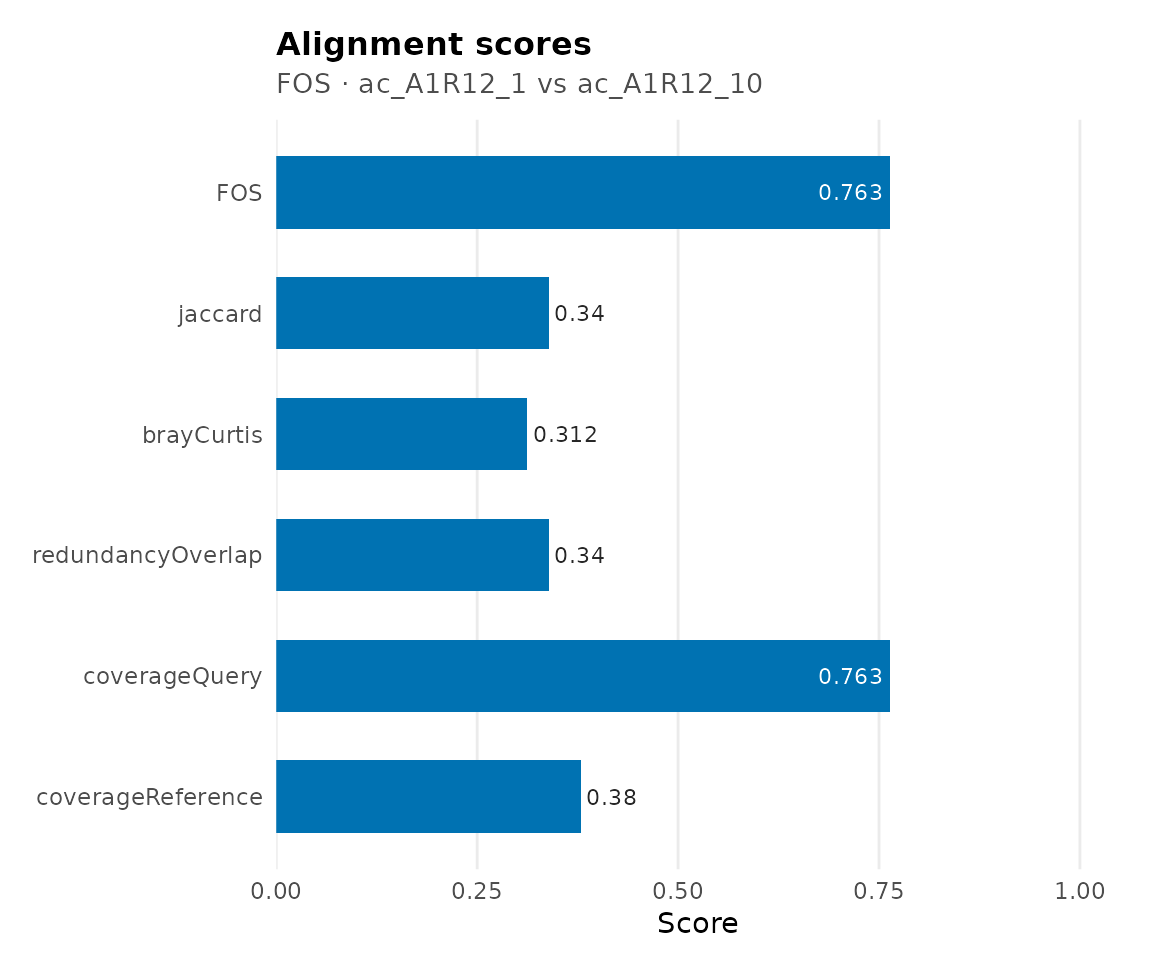
#> Pathways: 71 shared, 22 query-only, 116 reference-only.

Similarity metrics

Five metrics are available via the method argument. Regardless of which is selected as the primary score, all applicable metrics are always computed and stored.

cma_fos <- align(cm_list[[1]], cm_list[[2]], method = "FOS")
cma_jac <- align(cm_list[[1]], cm_list[[2]], method = "jaccard")
scores(cma_fos)
#> $FOS
#> [1] 0.7634409
#> 
#> $jaccard
#> [1] 0.3397129
#> 
#> $brayCurtis
#> [1] 0.3115158
#> 
#> $redundancyOverlap
#> [1] 0.3397129
#> 
#> $coverageQuery
#> [1] 0.7634409
#> 
#> $coverageReference
#> [1] 0.3796791

Metric	Description
FOS	Szymkiewicz-Simpson on binary matrices
Jaccard	Symmetric set similarity
Bray-Curtis	Flux-weighted similarity
Redundancy Overlap	Weighted Jaccard on nSpecies
MAAS	0.4 FOS + 0.2 each of the rest

The Metabolic Alignment Aggregate Score (MAAS) combines all four metrics. Weights are renormalised when some metrics are unavailable (e.g., unweighted networks lack Bray-Curtis):

cma_maas <- align(cm_list[[1]], cm_list[[2]], method = "MAAS")
scores(cma_maas)
#> $FOS
#> [1] 0.7634409
#> 
#> $jaccard
#> [1] 0.3397129
#> 
#> $brayCurtis
#> [1] 0.3115158
#> 
#> $redundancyOverlap
#> [1] 0.3397129
#> 
#> $coverageQuery
#> [1] 0.7634409
#> 
#> $coverageReference
#> [1] 0.3796791
#> 
#> $MAAS
#> [1] 0.5035647

The FOS subset property

FOS uses the Szymkiewicz-Simpson coefficient, which divides by the smaller network. This means FOS = 1 whenever a small consortium is a strict functional subset of a larger one – even if the larger consortium has many additional pathways.

To detect this, ramen reports coverage ratios alongside the similarity metrics:

scores(cma_fos)[c("FOS", "coverageQuery", "coverageReference")]
#> $FOS
#> [1] 0.7634409
#> 
#> $coverageQuery
#> [1] 0.7634409
#> 
#> $coverageReference
#> [1] 0.3796791

coverageQuery: fraction of the query’s pathways found in the reference
coverageReference: fraction of the reference’s pathways found in the query

When FOS is high but one coverage ratio is low, the alignment represents a subset relationship rather than true functional equivalence. For symmetric similarity, use Jaccard instead.

Pathway correspondences

The alignment classifies every metabolite-to-metabolite pathway as shared, unique to the query, or unique to the reference.

## All pathways in the alignment
head(pathways(cma))
#> # A tibble: 6 × 2
#>   consumed produced
#>   <chr>    <chr>   
#> 1 acald    ac      
#> 2 asp__L   ac      
#> 3 gly      ac      
#> 4 gthrd    ac      
#> 5 h2o2     ac      
#> 6 h2s      ac

## Shared pathways only
shared <- pathways(cma, type = "shared")
nrow(shared)
#> [1] 71

## Unique pathways (returns a list with $query and $reference)
unique_pw <- pathways(cma, type = "unique")
nrow(unique_pw$query)
#> [1] 22
nrow(unique_pw$reference)
#> [1] 116

Permutation p-values

Statistical significance is assessed by degree-preserving network rewiring. The query network’s pathways are shuffled while preserving each metabolite’s degree, and the metric is recomputed under the null distribution. For MAAS, only the binary network topology is permuted; the weighted assays (Consumption, Production, nSpecies) remain fixed, so the null distribution reflects topological variation in the composite score.

cma_p <- align(
    cm_list[[1]],
    cm_list[[2]],
    method = "FOS",
    computePvalue = TRUE,
    nPermutations = 99L
)
scores(cma_p)
#> $FOS
#> [1] 0.7634409
#> 
#> $jaccard
#> [1] 0.3397129
#> 
#> $brayCurtis
#> [1] 0.3115158
#> 
#> $redundancyOverlap
#> [1] 0.3397129
#> 
#> $coverageQuery
#> [1] 0.7634409
#> 
#> $coverageReference
#> [1] 0.3796791
#> 
#> $pvalue
#> [1] 0.01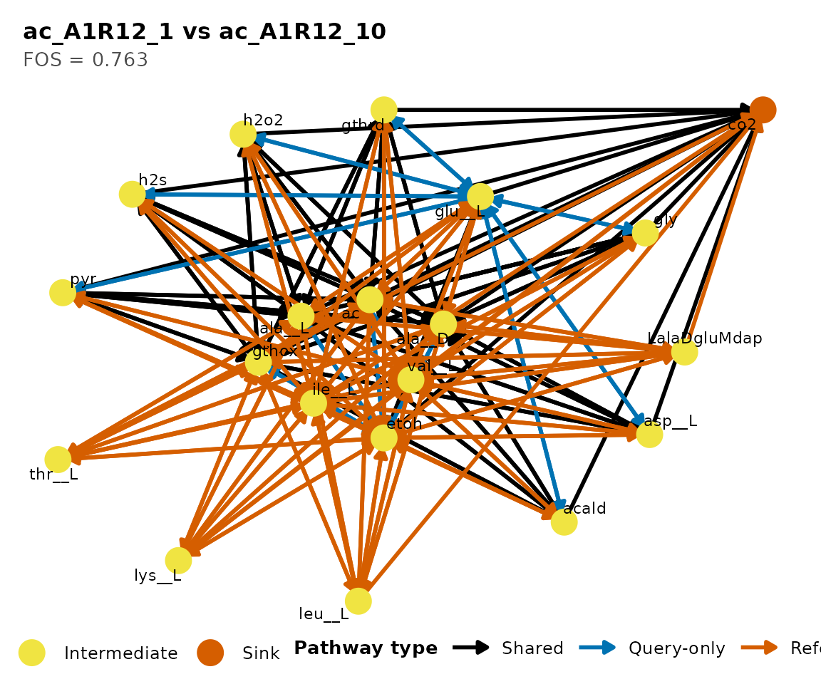

Visualisation

Network plot

The network view shows shared (green), query-unique (blue), and reference-unique (red) pathways as a directed metabolite flow graph.

plot(cma, type = "network")

Pairwise alignment network.

Score bar chart

plot(cma, type = "scores")

Pairwise metric scores.

Multiple alignment

Aligning a consortium set

align(CMS) computes pairwise similarities across all consortia in a ConsortiumMetabolismSet and returns a CMA with Type = "multiple".

cma_mult <- align(cms)
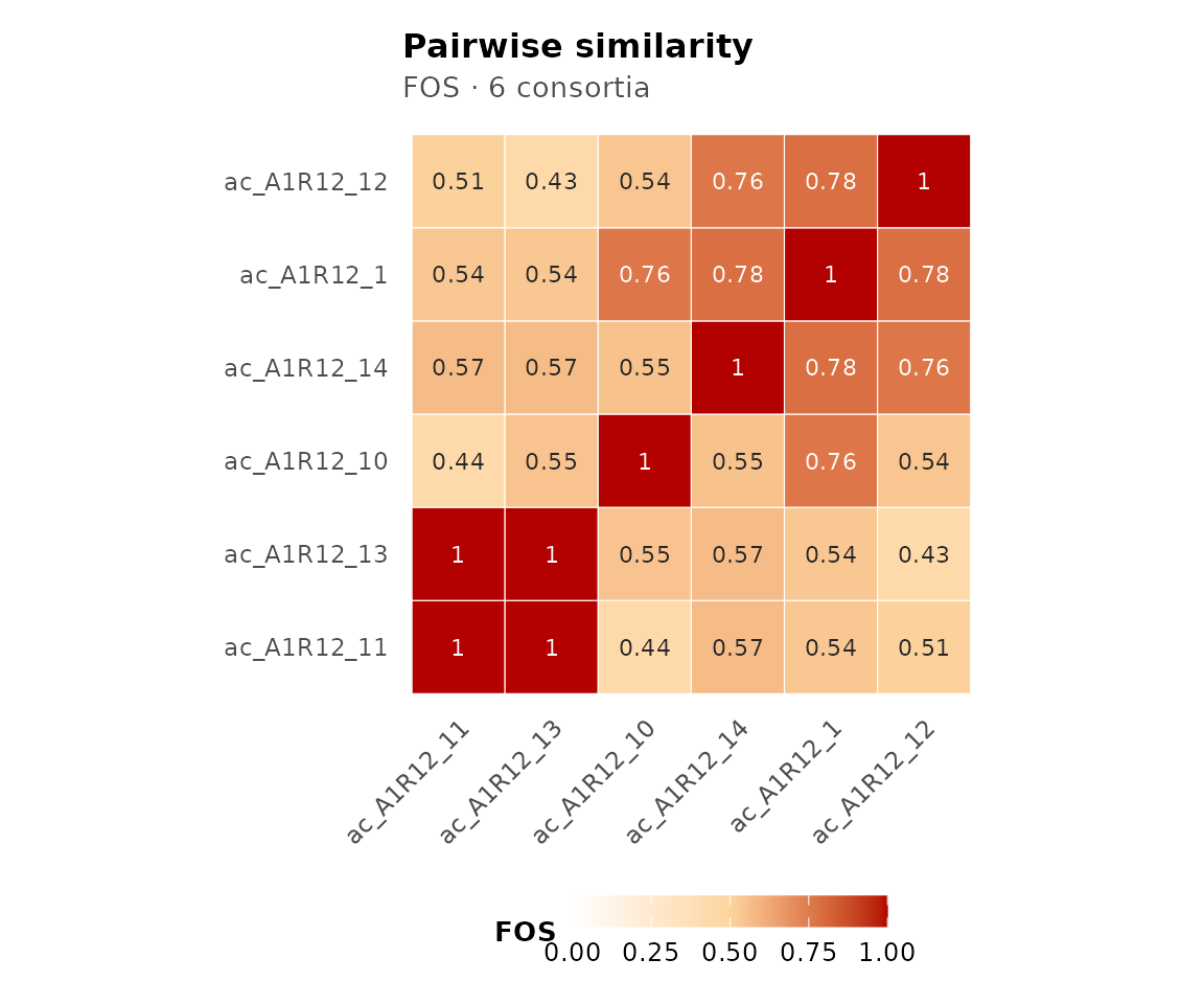
cma_mult

Similarity matrix

The similarity matrix is an n x n symmetric matrix with 1s on the diagonal. For FOS, this is derived from the pre-computed CMS overlap matrix:

round(similarityMatrix(cma_mult), 3)
#>             ac_A1R12_1 ac_A1R12_10 ac_A1R12_11 ac_A1R12_12 ac_A1R12_13
#> ac_A1R12_1       1.000       0.763       0.538       0.785       0.538
#> ac_A1R12_10      0.763       1.000       0.438       0.542       0.549
#> ac_A1R12_11      0.538       0.438       1.000       0.507       1.000
#> ac_A1R12_12      0.785       0.542       0.507       1.000       0.430
#> ac_A1R12_13      0.538       0.549       1.000       0.430       1.000
#> ac_A1R12_14      0.785       0.551       0.567       0.764       0.567
#>             ac_A1R12_14
#> ac_A1R12_1        0.785
#> ac_A1R12_10       0.551
#> ac_A1R12_11       0.567
#> ac_A1R12_12       0.764
#> ac_A1R12_13       0.567
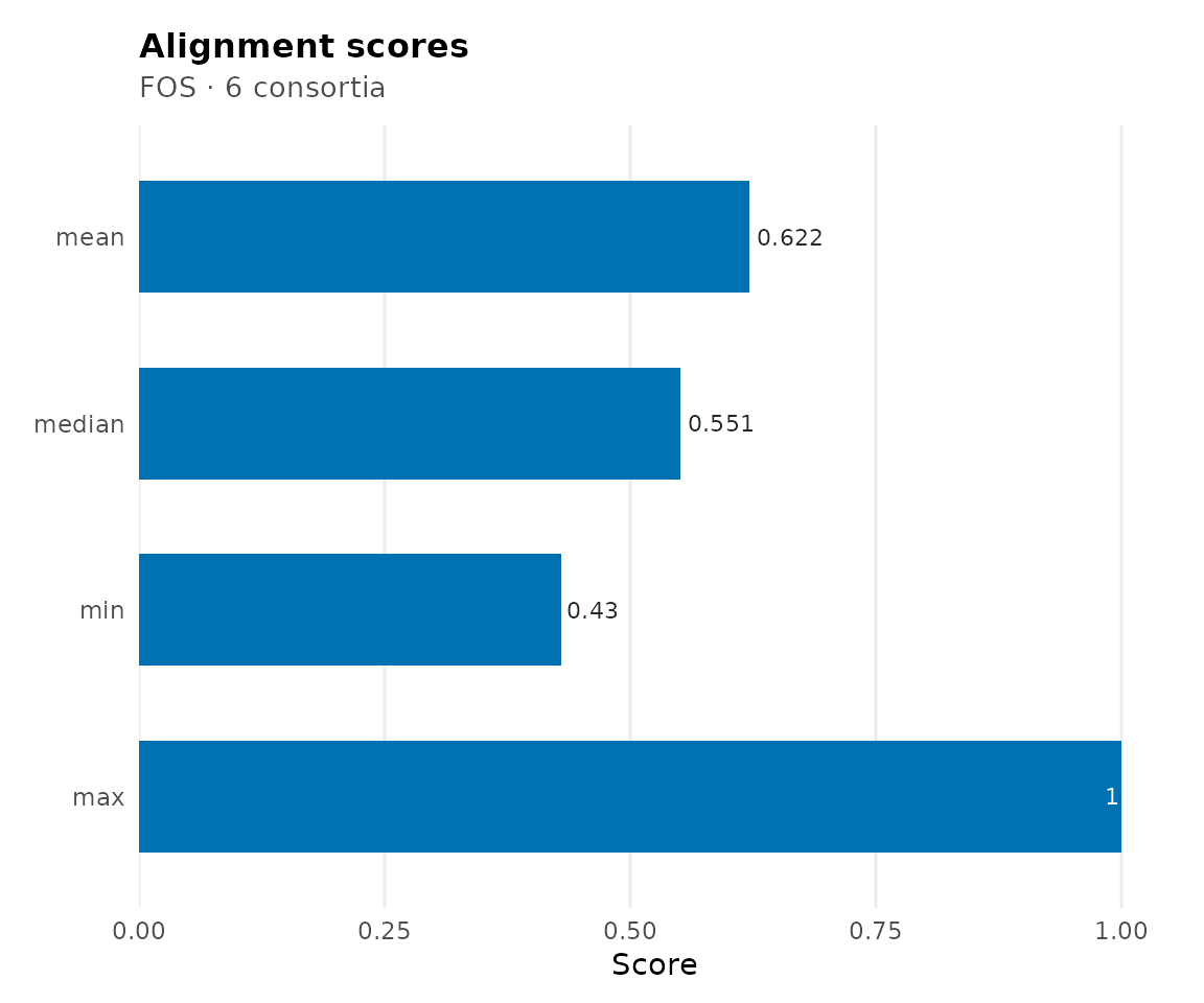
#> ac_A1R12_14       1.000

Summary scores

For a multiple alignment, the primary score is the median of all pairwise scores. scores() returns full summary statistics:

scores(cma_mult)
#> $mean
#> [1] 0.6215862
#> 
#> $median
#> [1] 0.5511811
#> 
#> $min
#> [1] 0.4295775
#> 
#> $max
#> [1] 1
#> 
#> $sd
#> [1] 0.1597042
#> 
#> $nPairs
#> [1] 15

Consensus network and prevalence

Pathway prevalence counts how many consortia share each metabolite-to-metabolite pathway. This enables classification of pathways as core (present in most consortia) or niche (present in few).

prev <- prevalence(cma_mult)
head(prev[order(-prev$nConsortia), ])
#>    consumed produced nConsortia proportion
#> 21   asp__L       ac          6          1
#> 24      gly       ac          6          1
#> 30      pyr       ac          6          1
#> 56   asp__L   ala__D          6          1
#> 59      gly   ala__D          6          1
#> 65      pyr   ala__D          6          1

## Distribution of prevalence
table(prev$nConsortia)
#> 
#>   1   2   3   4   5   6 
#> 100  75  55  51  14  30

The pathways() method with type = "consensus" returns the same information:

head(pathways(cma_mult, type = "consensus"))
#>   consumed produced nConsortia proportion
#> 1    acald    4abut          1  0.1666667
#> 2   arg__L    4abut          1  0.1666667
#> 3   asp__L    4abut          1  0.1666667
#> 4     etoh    4abut          1  0.1666667
#> 5      gly    4abut          1  0.1666667
#> 6   leu__L    4abut          1  0.1666667

Visualisation

Heatmap

The heatmap shows pairwise similarities with dendrogram-based ordering:

plot(cma_mult, type = "heatmap")

Similarity heatmap.

Score summary

plot(cma_mult, type = "scores")

Multiple alignment summary scores.

Database search

align(CM, CMS) compares a single query consortium against every member of a set and returns a CMA with Type = "search". This is the natural call for questions like “which consortium in my database is most functionally similar to this query?”

Basic search

We hold out the first consortium as a query and search it against a database built from the remaining five:

query <- cm_list[[1]]
db <- ConsortiumMetabolismSet(cm_list[-1], name = "db")

hits <- align(query, db)
#> Searching 5 consortia using "FOS".
hits
#> 
#> ── ConsortiumMetabolismAlignment 
#> Name: "ac_A1R12_1 vs CMS (5 consortia)"
#> Type: "search"
#> Metric: "FOS"
#> Score: 0.7849
#> Query: "ac_A1R12_1", Top hit: "ac_A1R12_12" (of 5 consortia)

The top-hit name and score sit on ReferenceName / PrimaryScore. The full ranked table is stored in Scores$ranking:

ranking <- scores(hits)$ranking
head(ranking)
#> # A tibble: 5 × 8
#>   reference   score   FOS jaccard brayCurtis redundancyOverlap coverageQuery
#>   <chr>       <dbl> <dbl>   <dbl>      <dbl>             <dbl>         <dbl>
#> 1 ac_A1R12_12 0.785 0.785   0.451      0.635             0.451         0.785
#> 2 ac_A1R12_14 0.785 0.785   0.497      0.553             0.497         0.785
#> 3 ac_A1R12_10 0.763 0.763   0.340      0.312             0.340         0.763
#> 4 ac_A1R12_11 0.538 0.538   0.226      0.500             0.226         0.538
#> 5 ac_A1R12_13 0.538 0.538   0.270      0.515             0.270         0.538
#> # ℹ 1 more variable: coverageReference <dbl>

Each row holds the reference consortium’s name, the primary score (under the requested method), all four individual metric columns, and the coverage ratios against the query. Rows are pre-sorted by score in descending order.

Top-K hits

Use topK to truncate the ranked table – useful when the database is large and only the best matches matter:

hits_top3 <- align(query, db, topK = 3L)
#> Searching 5 consortia using "FOS".
scores(hits_top3)$ranking
#> # A tibble: 3 × 8
#>   reference   score   FOS jaccard brayCurtis redundancyOverlap coverageQuery
#>   <chr>       <dbl> <dbl>   <dbl>      <dbl>             <dbl>         <dbl>
#> 1 ac_A1R12_12 0.785 0.785   0.451      0.635             0.451         0.785
#> 2 ac_A1R12_14 0.785 0.785   0.497      0.553             0.497         0.785
#> 3 ac_A1R12_10 0.763 0.763   0.340      0.312             0.340         0.763
#> # ℹ 1 more variable: coverageReference <dbl>

similarityMatrix() returns a 1 x n row vector (or 1 x topK if truncated), with the query name as the row label:

round(similarityMatrix(hits_top3), 3)
#>            ac_A1R12_12 ac_A1R12_14 ac_A1R12_10
#> ac_A1R12_1       0.785       0.785       0.763

Pathway correspondences always reflect the single overall top hit, regardless of topK:

head(pathways(hits_top3, type = "shared"))
#> # A tibble: 6 × 2
#>   consumed produced
#>   <chr>    <chr>   
#> 1 asp__L   ac      
#> 2 etoh     ac      
#> 3 gly      ac      
#> 4 gthrd    ac      
#> 5 h2o2     ac      
#> 6 pyr      ac

Choosing metrics

By default all four base metrics are computed for every database member. For large databases, restricting metrics skips the weighted-assay expansion and can be substantially faster:

hits_fos <- align(query, db, metrics = "FOS")
#> Searching 5 consortia using "FOS".
scores(hits_fos)$ranking[,
    c("reference", "score", "brayCurtis")
]
#> # A tibble: 5 × 3
#>   reference   score brayCurtis
#>   <chr>       <dbl>      <dbl>
#> 1 ac_A1R12_12 0.785         NA
#> 2 ac_A1R12_14 0.785         NA
#> 3 ac_A1R12_10 0.763         NA
#> 4 ac_A1R12_11 0.538         NA
#> 5 ac_A1R12_13 0.538         NA

Columns for skipped metrics remain in the ranking table but are filled with NA, making the schema stable across calls.

Significance of the top hit

As in pairwise alignment, computePvalue = TRUE runs a degree-preserving permutation test. For database search, the test is applied only to the top hit – a BLAST-style convention that keeps the cost comparable to a single pairwise p-value:

hits_p <- align(
    query,
    db,
    computePvalue = TRUE,
    nPermutations = 99L
)
#> Searching 5 consortia using "FOS".
hits_p
#> 
#> ── ConsortiumMetabolismAlignment 
#> Name: "ac_A1R12_1 vs CMS (5 consortia)"
#> Type: "search"
#> Metric: "FOS"
#> Score: 0.7849
#> P-value: "0.01"
#> Query: "ac_A1R12_1", Top hit: "ac_A1R12_12" (of 5 consortia)

The show() output reports the top hit, its score, and the p-value directly; scores(hits_p) gives the full numeric breakdown including pvalue.

If statistical confidence is needed for several top hits, re-run align() in pairwise mode against each candidate individually.

Accessor reference

Accessor	Alignment type	Returns
`scores()`	all	Named list of scores (+ `$ranking` for search)
`pathways()`	all	data.frame of all pathways
`pathways(type = "shared")`	pairwise, search	shared pathways
`pathways(type = "unique")`	pairwise, search	list(query, reference)
`pathways(type = "consensus")`	multiple	data.frame with prevalence
`similarityMatrix()`	multiple, search	n x n or 1 x n numeric matrix
`prevalence()`	multiple	data.frame with nConsortia
`metabolites()`	all	Character vector of metabolites

Type guards prevent misuse – for example, calling pathways(type = "consensus") on a pairwise alignment raises an informative error.

Session info

sessionInfo()
#> R version 4.6.0 (2026-04-24)
#> Platform: x86_64-pc-linux-gnu
#> Running under: Ubuntu 24.04.4 LTS
#> 
#> Matrix products: default
#> BLAS:   /usr/lib/x86_64-linux-gnu/openblas-pthread/libblas.so.3 
#> LAPACK: /usr/lib/x86_64-linux-gnu/openblas-pthread/libopenblasp-r0.3.26.so;  LAPACK version 3.12.0
#> 
#> locale:
#>  [1] LC_CTYPE=C.UTF-8       LC_NUMERIC=C           LC_TIME=C.UTF-8       
#>  [4] LC_COLLATE=C.UTF-8     LC_MONETARY=C.UTF-8    LC_MESSAGES=C.UTF-8   
#>  [7] LC_PAPER=C.UTF-8       LC_NAME=C              LC_ADDRESS=C          
#> [10] LC_TELEPHONE=C         LC_MEASUREMENT=C.UTF-8 LC_IDENTIFICATION=C   
#> 
#> time zone: UTC
#> tzcode source: system (glibc)
#> 
#> attached base packages:
#> [1] stats     graphics  grDevices utils     datasets  methods   base     
#> 
#> other attached packages:
#> [1] ramen_0.99.0     BiocStyle_2.40.0
#> 
#> loaded via a namespace (and not attached):
#>  [1] tidyselect_1.2.1                viridisLite_0.4.3              
#>  [3] dplyr_1.2.1                     farver_2.1.2                   
#>  [5] viridis_0.6.5                   Biostrings_2.80.0              
#>  [7] S7_0.2.2                        ggraph_2.2.2                   
#>  [9] fastmap_1.2.0                   SingleCellExperiment_1.34.0    
#> [11] lazyeval_0.2.3                  tweenr_2.0.3                   
#> [13] digest_0.6.39                   lifecycle_1.0.5                
#> [15] tidytree_0.4.7                  magrittr_2.0.5                 
#> [17] compiler_4.6.0                  rlang_1.2.0                    
#> [19] sass_0.4.10                     tools_4.6.0                    
#> [21] utf8_1.2.6                      igraph_2.3.1                   
#> [23] yaml_2.3.12                     knitr_1.51                     
#> [25] labeling_0.4.3                  graphlayouts_1.2.3             
#> [27] S4Arrays_1.12.0                 DelayedArray_0.38.1            
#> [29] RColorBrewer_1.1-3              TreeSummarizedExperiment_2.20.0
#> [31] abind_1.4-8                     BiocParallel_1.46.0            
#> [33] withr_3.0.2                     purrr_1.2.2                    
#> [35] BiocGenerics_0.58.0             desc_1.4.3                     
#> [37] grid_4.6.0                      polyclip_1.10-7                
#> [39] stats4_4.6.0                    ggplot2_4.0.3                  
#> [41] scales_1.4.0                    MASS_7.3-65                    
#> [43] SummarizedExperiment_1.42.0     cli_3.6.6                      
#> [45] rmarkdown_2.31                  crayon_1.5.3                   
#> [47] ragg_1.5.2                      treeio_1.36.1                  
#> [49] generics_0.1.4                  ape_5.8-1                      
#> [51] cachem_1.1.0                    ggforce_0.5.0                  
#> [53] parallel_4.6.0                  BiocManager_1.30.27            
#> [55] XVector_0.52.0                  matrixStats_1.5.0              
#> [57] vctrs_0.7.3                     yulab.utils_0.2.4              
#> [59] Matrix_1.7-5                    jsonlite_2.0.0                 
#> [61] bookdown_0.46                   IRanges_2.46.0                 
#> [63] S4Vectors_0.50.0                ggrepel_0.9.8                  
#> [65] systemfonts_1.3.2               dendextend_1.19.1              
#> [67] tidyr_1.3.2                     jquerylib_0.1.4                
#> [69] glue_1.8.1                      pkgdown_2.2.0                  
#> [71] codetools_0.2-20                gtable_0.3.6                   
#> [73] GenomicRanges_1.64.0            tibble_3.3.1                   
#> [75] pillar_1.11.1                   rappdirs_0.3.4                 
#> [77] htmltools_0.5.9                 Seqinfo_1.2.0                  
#> [79] R6_2.6.1                        textshaping_1.0.5              
#> [81] tidygraph_1.3.1                 evaluate_1.0.5                 
#> [83] lattice_0.22-9                  Biobase_2.72.0                 
#> [85] memoise_2.0.1                   bslib_0.10.0                   
#> [87] Rcpp_1.1.1-1.1                  gridExtra_2.3                  
#> [89] SparseArray_1.12.2              nlme_3.1-169                   
#> [91] xfun_0.57                       fs_2.1.0                       
#> [93] MatrixGenerics_1.24.0           pkgconfig_2.0.3