The ConsortiumMetabolismSet Class
Source:vignettes/ConsortiumMetabolismSet.Rmd
ConsortiumMetabolismSet.RmdIntroduction
The ConsortiumMetabolismSet (CMS) class groups multiple
ConsortiumMetabolism objects into a single analysis unit.
When a CMS is constructed, ramen automatically:
- Expands all binary matrices to a shared universal metabolite space
- Computes pairwise overlap scores (Functional Overlap Score) between every pair of consortia
- Builds a dendrogram via hierarchical clustering on the dissimilarity matrix (1 - overlap)
This vignette covers CMS construction, accessors, the overlap matrix, dendrogram operations, species and pathway classification, and cluster extraction.
Construction
From a list of CMs
The ConsortiumMetabolismSet() constructor accepts any
number of ConsortiumMetabolism objects (or a list of them),
plus a name.
cm_alpha <- synCM("Alpha", n_species = 5, max_met = 10, seed = 42)
cm_beta <- synCM("Beta", n_species = 5, max_met = 10, seed = 43)
cm_gamma <- synCM("Gamma", n_species = 4, max_met = 8, seed = 44)
cm_delta <- synCM("Delta", n_species = 6, max_met = 10, seed = 45)

cms_syn <- ConsortiumMetabolismSet(
    cm_alpha, cm_beta, cm_gamma, cm_delta,
    name = "SyntheticSet"
)
cms_syn
A list of CMs works equally well:
cm_list <- list(cm_alpha, cm_beta)
cms_small <- ConsortiumMetabolismSet(
    cm_list,
    name = "SmallSet"
)
cms_small
From MiSoSoup data
The misosoup24 dataset contains 56 metabolic solutions.
Here we construct CMs from the first four and combine them into a
CMS.
data("misosoup24")

## Build 4 CMs from the dataset
cm_ms <- lapply(seq_len(4), function(i) {
    ConsortiumMetabolism(
        misosoup24[[i]],
        name = names(misosoup24)[i],
        species_col = "species",
        metabolite_col = "metabolites",
        flux_col = "fluxes"
    )
})

cms_ms <- ConsortiumMetabolismSet(
    cm_ms,
    name = "MiSoSoup_subset"
)
cms_ms
The show() method
Printing a CMS displays the name, the number of consortia, and the description.
cms_syn
#>
#> ── ConsortiumMetabolismSet
#> Name: "SyntheticSet"
#> Containing 4 consortia.
#> Description: NA
Accessors
name() and description()
name(cms_syn)
#> [1] "SyntheticSet"
description(cms_syn)
#> [1] NA
species()
For a CMS, species() returns a tibble of all species
across consortia with the number of distinct pathways each species
catalyses, sorted in descending order.
species(cms_syn)
#> # A tibble: 20 × 2
#>    species  n_pathways
#>    <chr>         <int>
#>  1 HRC7700N         21
#>  2 IEV6830P         20
#>  3 DKC1921L         20
#>  4 QWK6670F         18
#>  5 TDU2395Q         16
#>  6 NZU3486L         15
#>  7 SZW1907Q         12
#>  8 IAJ4395F         12
#>  9 PYQ2630S         10
#> 10 GGM5859Q          9
#> 11 MEU9286A          6
#> 12 FMD9122E          6
#> 13 VYI1693V          4
#> 14 XPH2498O          4
#> 15 BJV7623S          3
#> 16 WEL6294Y          2
#> 17 BDN9096E          2
#> 18 OCP8184Z          2
#> 19 MUN1889P          1
#> 20 TAF9777Y          1
metabolites()
Returns a sorted character vector of all metabolites across the universal metabolite space.
metabolites(cms_syn)
#>  [1] "met1"  "met10" "met2"  "met3"  "met4"  "met5"  "met6"  "met7"  "met8"
#> [10] "met9"Overlap matrix
The overlap matrix stores pairwise dissimilarity scores (1 - Functional Overlap Score) between all consortia. The FOS is the Szymkiewicz-Simpson coefficient applied to the binary metabolite-metabolite matrices.
cms_syn@OverlapMatrix
#>           Alpha      Beta     Gamma     Delta
#> Alpha 0.0000000 0.5526316 0.4444444 0.4615385
#> Beta  0.5526316 0.0000000 0.5185185 0.4736842
#> Gamma 0.4444444 0.5185185 0.0000000 0.5185185
#> Delta 0.4615385 0.4736842 0.5185185 0.0000000
Values near 0 on the diagonal indicate self-identity; off-diagonal values close to 0 mean high similarity.
Dendrogram
The dendrogram is built from the overlap (dissimilarity) matrix using
hierarchical clustering and is stored in the Dendrogram
slot.
dend <- cms_syn@Dendrogram[[1]]
plot(dend, main = "Consortium dendrogram")
The NodeData slot contains the positions of internal
dendrogram nodes, which are used by extractCluster() and
plot().
cms_syn@NodeData
#> # A tibble: 3 × 4
#>       x     y original_node_id node_id
#>   <dbl> <dbl>            <int>   <int>
#> 1   2.5 0.785                1       1
#> 2   3.5 0.676                5       2
#> 3   1.5 0.632                2       3
Pathway classification
The pathways() method with a type argument
classifies pathways by prevalence across consortia or species.
Pan-consortia pathways
Pathways present in many consortia (top fraction).
pathways(cms_syn, type = "pan-cons")
#> # A tibble: 4 × 4
#>   consumed produced n_species n_cons
#>   <chr>    <chr>        <int>  <int>
#> 1 met7     met2             5      4
#> 2 met1     met5             4      4
#> 3 met1     met2             4      4
#> 4 met1     met8             6      4
Niche pathways
Pathways present in few consortia (bottom fraction).
pathways(cms_syn, type = "niche")
#> # A tibble: 32 × 4
#>    consumed produced n_species n_cons
#>    <chr>    <chr>        <int>  <int>
#>  1 met2     met1             1      1
#>  2 met2     met7             1      1
#>  3 met2     met4             1      1
#>  4 met8     met1             1      1
#>  5 met4     met5             1      1
#>  6 met10    met4             1      1
#>  7 met10    met6             1      1
#>  8 met10    met2             1      1
#>  9 met10    met5             1      1
#> 10 met10    met1             1      1
#> # ℹ 22 more rows
Core pathways
Pathways catalysed by many species (top fraction).
pathways(cms_syn, type = "core")
#> # A tibble: 0 × 4
#> # ℹ 4 variables: consumed <chr>, produced <chr>, n_species <int>, n_cons <int>
Auxiliary pathways
Pathways catalysed by few species (bottom fraction).
pathways(cms_syn, type = "aux")
#> # A tibble: 46 × 4
#>    consumed produced n_species n_cons
#>    <chr>    <chr>        <int>  <int>
#>  1 met2     met1             1      1
#>  2 met2     met7             1      1
#>  3 met2     met4             1      1
#>  4 met8     met1             1      1
#>  5 met4     met5             1      1
#>  6 met10    met4             1      1
#>  7 met10    met6             1      1
#>  8 met10    met2             1      1
#>  9 met10    met5             1      1
#> 10 met10    met1             1      1
#> # ℹ 36 more rows
The quantileCutoff parameter controls the threshold
(default 0.1).
Species classification
The species() method for CMS supports filtering by
metabolic role.
Generalists
Species with the most distinct pathways (top 15% by default).
species(cms_syn, type = "generalists")
#> # A tibble: 3 × 2
#>   species  n_pathways
#>   <chr>         <int>
#> 1 HRC7700N         21
#> 2 IEV6830P         20
#> 3 DKC1921L         20
Specialists
Species with the fewest distinct pathways (bottom 15% by default).
species(cms_syn, type = "specialists")
#> # A tibble: 3 × 2
#>   species  n_pathways
#>   <chr>         <int>
#> 1 OCP8184Z          2
#> 2 MUN1889P          1
#> 3 TAF9777Y          1
The quantileCutoff parameter adjusts the fraction:
species(cms_syn, type = "generalists", quantileCutoff = 0.25)
#> # A tibble: 5 × 2
#>   species  n_pathways
#>   <chr>         <int>
#> 1 HRC7700N         21
#> 2 IEV6830P         20
#> 3 DKC1921L         20
#> 4 QWK6670F         18
#> 5 TDU2395Q         16
Functional groups
functionalGroups() computes pairwise Jaccard
similarities between species based on their pathway sets, performs
hierarchical clustering, and returns a dendrogram coloured by
k groups.
fg <- functionalGroups(cms_syn, k = 3)
#> Loading required namespace: colorspace
#> Warning: Using `size` aesthetic for lines was deprecated in ggplot2 3.4.0.
#> ℹ Please use `linewidth` instead.
#> ℹ The deprecated feature was likely used in the dendextend package.
#>   Please report the issue at <https://github.com/talgalili/dendextend/issues>.
#> This warning is displayed once per session.
#> Call `lifecycle::last_lifecycle_warnings()` to see where this warning was
#> generated.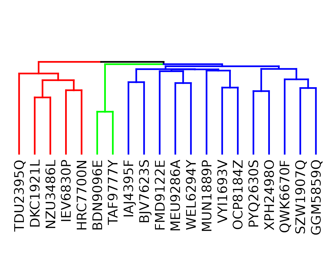
Functional groups dendrogram.
The returned list (invisible) contains the plot, dendrogram, similarity matrix, species combinations, and per-species reaction sets:
names(fg)
#> [1] "plot"                  "dendrogram"            "similarity_matrix"
#> [4] "species_combinations"  "reactions_per_species"
Cluster extraction
Given the numbered internal nodes visible in plot(cms)
or NodeData, extractCluster() pulls out a
sub-CMS containing only the consortia under a given node.
sub_cms <- extractCluster(cms_syn, node_id = 1)
sub_cms
Replacement methods
description<-
description(cms_syn) <- "Four synthetic consortia"
description(cms_syn)
#> [1] "Four synthetic consortia"
Session info
sessionInfo()
#> R version 4.5.3 (2026-03-11)
#> Platform: x86_64-pc-linux-gnu
#> Running under: Ubuntu 24.04.4 LTS
#>
#> Matrix products: default
#> BLAS:   /usr/lib/x86_64-linux-gnu/openblas-pthread/libblas.so.3
#> LAPACK: /usr/lib/x86_64-linux-gnu/openblas-pthread/libopenblasp-r0.3.26.so;  LAPACK version 3.12.0
#>
#> locale:
#>  [1] LC_CTYPE=C.UTF-8       LC_NUMERIC=C           LC_TIME=C.UTF-8
#>  [4] LC_COLLATE=C.UTF-8     LC_MONETARY=C.UTF-8    LC_MESSAGES=C.UTF-8
#>  [7] LC_PAPER=C.UTF-8       LC_NAME=C              LC_ADDRESS=C
#> [10] LC_TELEPHONE=C         LC_MEASUREMENT=C.UTF-8 LC_IDENTIFICATION=C
#>
#> time zone: UTC
#> tzcode source: system (glibc)
#>
#> attached base packages:
#> [1] stats     graphics  grDevices utils     datasets  methods   base
#>
#> other attached packages:
#> [1] ramen_0.0.0.9001 BiocStyle_2.38.0
#>
#> loaded via a namespace (and not attached):
#>  [1] SummarizedExperiment_1.40.0     gtable_0.3.6
#>  [3] ggplot2_4.0.2                   xfun_0.57
#>  [5] bslib_0.10.0                    Biobase_2.70.0
#>  [7] lattice_0.22-9                  yulab.utils_0.2.4
#>  [9] vctrs_0.7.2                     tools_4.5.3
#> [11] generics_0.1.4                  stats4_4.5.3
#> [13] parallel_4.5.3                  tibble_3.3.1
#> [15] pkgconfig_2.0.3                 Matrix_1.7-4
#> [17] RColorBrewer_1.1-3              S7_0.2.1
#> [19] desc_1.4.3                      S4Vectors_0.48.0
#> [21] lifecycle_1.0.5                 farver_2.1.2
#> [23] compiler_4.5.3                  treeio_1.34.0
#> [25] textshaping_1.0.5               Biostrings_2.78.0
#> [27] Seqinfo_1.0.0                   codetools_0.2-20
#> [29] htmltools_0.5.9                 sass_0.4.10
#> [31] yaml_2.3.12                     lazyeval_0.2.2
#> [33] pkgdown_2.2.0                   pillar_1.11.1
#> [35] crayon_1.5.3                    jquerylib_0.1.4
#> [37] tidyr_1.3.2                     BiocParallel_1.44.0
#> [39] SingleCellExperiment_1.32.0     DelayedArray_0.36.0
#> [41] cachem_1.1.0                    viridis_0.6.5
#> [43] abind_1.4-8                     nlme_3.1-168
#> [45] tidyselect_1.2.1                digest_0.6.39
#> [47] dplyr_1.2.0                     purrr_1.2.1
#> [49] bookdown_0.46                   labeling_0.4.3
#> [51] TreeSummarizedExperiment_2.18.0 fastmap_1.2.0
#> [53] grid_4.5.3                      cli_3.6.5
#> [55] SparseArray_1.10.10             magrittr_2.0.4
#> [57] S4Arrays_1.10.1                 utf8_1.2.6
#> [59] ape_5.8-1                       withr_3.0.2
#> [61] scales_1.4.0                    rappdirs_0.3.4
#> [63] rmarkdown_2.31                  XVector_0.50.0
#> [65] matrixStats_1.5.0               igraph_2.2.2
#> [67] gridExtra_2.3                   ragg_1.5.2
#> [69] evaluate_1.0.5                  knitr_1.51
#> [71] GenomicRanges_1.62.1            IRanges_2.44.0
#> [73] viridisLite_0.4.3               rlang_1.1.7
#> [75] dendextend_1.19.1               Rcpp_1.1.1
#> [77] glue_1.8.0                      tidytree_0.4.7
#> [79] BiocManager_1.30.27             BiocGenerics_0.56.0
#> [81] jsonlite_2.0.0                  R6_2.6.1
#> [83] MatrixGenerics_1.22.0           systemfonts_1.3.2
#> [85] fs_2.0.1